


本期我们使用dolfinx解决Poisson方程:
$$-\nabla^2 u =f\quad in\ \Omega$$
$$u=0\quad on\ \Gamma_D$$
$$\nabla u \cdot \vec{n}=g\quad on\ \Gamma_N$$
易得其变分形式为
$$\int_\Omega{\nabla u\cdot\nabla v}dxdy=\int_\Omega{fv}dxdy+\int_{\Gamma_N}{gv}ds.$$
边界为矩形区域,Dirichlet边界和Neumann边界如下
\(\Omega = [0,2] \times [0,1]\),
\(\Gamma_{D} = \{(0, y) \cup (2, y) \subset \partial \Omega\}\),
\(\Gamma_{N} = \{(x, 0) \cup (x, 1) \subset \partial \Omega\}\).
函数\(f, g\)分别定义为
\(f = 10\exp(-((x - 0.5)^2 + (y - 0.5)^2) / 0.02)\), \(g = \sin(5x)\).
dolfinx代码实现
# ---
# jupyter:
#   jupytext:
#     text_representation:
#       extension: .py
#       format_name: light
#       format_version: '1.5'
#       jupytext_version: 1.13.6
# ---

# # Poisson equation
#
# This demo is implemented in {download}`demo_poisson.py`. It
# illustrates how to:
#
# - Create a {py:class}`function space <dolfinx.fem.FunctionSpace>`
# - Solve a linear partial differential equation
#
# ## Equation and problem definition
#
# For a domain $\Omega \subset \mathbb{R}^n$ with boundary $\partial
# \Omega = \Gamma_{D} \cup \Gamma_{N}$, the Poisson equation with
# particular boundary conditions reads:
#
# $$
# \begin{align}
#   - \nabla^{2} u &= f \quad {\rm in} \ \Omega, \\
#   u &= 0 \quad {\rm on} \ \Gamma_{D}, \\
#   \nabla u \cdot n &= g \quad {\rm on} \ \Gamma_{N}. \\
# \end{align}
# $$
#
# where $f$ and $g$ are input data and $n$ denotes the outward directed
# boundary normal. The variational problem reads: find $u \in V$ such
# that
#
# $$
# a(u, v) = L(v) \quad \forall \ v \in V,
# $$
#
# where $V$ is a suitable function space and
#
# $$
# \begin{align}
#   a(u, v) &:= \int_{\Omega} \nabla u \cdot \nabla v \, {\rm d} x, \\
#   L(v)    &:= \int_{\Omega} f v \, {\rm d} x + \int_{\Gamma_{N}} g v \, {\rm d} s.
# \end{align}
# $$
#
# The expression $a(u, v)$ is the bilinear form and $L(v)$
# is the linear form. It is assumed that all functions in $V$
# satisfy the Dirichlet boundary conditions ($u = 0 \ {\rm on} \
# \Gamma_{D}$).
#
# In this demo we consider:
#
# - $\Omega = [0,2] \times [0,1]$ (a rectangle)
# - $\Gamma_{D} = \{(0, y) \cup (2, y) \subset \partial \Omega\}$
# - $\Gamma_{N} = \{(x, 0) \cup (x, 1) \subset \partial \Omega\}$
# - $g = \sin(5x)$
# - $f = 10\exp(-((x - 0.5)^2 + (y - 0.5)^2) / 0.02)$
#   网格定义在二维网格[0, 2] * [0, 1]
#   Dirichlet边界是x=0, x=2(y in \Omega)
#   Neumann边界是y=0, 1(x in \Omega)

# ## Implementation
#
# The modules that will be used are imported:
#
import importlib.util

if importlib.util.find_spec("petsc4py") is not None:
    import dolfinx
    # Review: petsc4py是一个解线性方程组的包
    if not dolfinx.has_petsc:
        print("This demo requires DOLFINx to be compiled with PETSc enabled.")
        exit(0)
    from petsc4py.PETSc import ScalarType  # type: ignore
else:
    print("This demo requires petsc4py.")
    exit(0)

from mpi4py import MPI

# +
import numpy as np

import ufl
# UFL(Unified Form Language)是一个用于统一描述变分形式的 Python 库,在有限元方法(FEM)的数值计算中起着关键作用。
# 它由 FEniCS 项目开发,能让用户以接近数学公式的自然方式来表达变分问题,然后自动将这些表达式转换为适合数值求解的形式。
from dolfinx import fem, io, mesh, plot
from dolfinx.fem.petsc import LinearProblem
from ufl import ds, dx, grad, inner

# -

# Note that it is important to first `from mpi4py import MPI` to
# ensure that MPI is correctly initialised.

# We create a rectangular {py:class}`Mesh <dolfinx.mesh.Mesh>` using
# {py:func}`create_rectangle <dolfinx.mesh.create_rectangle>`, and
# create a finite element {py:class}`function space
# <dolfinx.fem.FunctionSpace>` $V$ on the mesh.

# +
# 创建计算区域
#
msh = mesh.create_rectangle(
    comm=MPI.COMM_WORLD,
    points=((0.0, 0.0), (2.0, 1.0)),
    n=(32, 16),
    cell_type=mesh.CellType.triangle,
)
# 设置函数空间 第二个参数 tuple:(family, degree)
# family表示有限元家族
# degree表示多项式的自由度 v是自由度为1的连续Lagrange有限元空间
V = fem.functionspace(msh, ("Lagrange", 1))
# -

# The second argument to {py:func}`functionspace
# <dolfinx.fem.functionspace>` is a tuple `(family, degree)`, where
# `family` is the finite element family, and `degree` specifies the
# polynomial degree. In this case `V` is a space of continuous Lagrange
# finite elements of degree 1.
#
# To apply the Dirichlet boundary conditions, we find the mesh facets
# (entities of topological co-dimension 1) that lie on the boundary
# $\Gamma_D$ using {py:func}`locate_entities_boundary
# <dolfinx.mesh.locate_entities_boundary>`. The function is provided
# with a 'marker' function that returns `True` for points `x` on the
# boundary and `False` otherwise.

# 设置Dirichlet边界条件
# 二维网格的边界是一段封闭曲线
# 一维网格的边界是左端点 和 右端点(本例)
# marker函数对 在边界上的x 返回True 反之 返回False
# np.isclose 是 NumPy 库中的一个函数,用于比较两个数组的元素是否在一定的容差范围内接近相等。
# 在处理浮点数比较时,由于浮点数在计算机中的存储方式可能会导致微小的误差,直接使用 == 进行比较可能会得到意外的结果
facets = mesh.locate_entities_boundary(
    msh,
    dim=(msh.topology.dim - 1),
    marker=lambda x: np.isclose(x[0], 0.0) | np.isclose(x[0], 2.0),
)


# We now find the degrees-of-freedom that are associated with the
# boundary facets using {py:func}`locate_dofs_topological
# <dolfinx.fem.locate_dofs_topological>`:

# 用于通过拓扑信息来定位自由度
# Return dofs 数组包含与指定边界面相关的自由度的编号。
dofs = fem.locate_dofs_topological(V=V, entity_dim=1, entities=facets)

# and use {py:func}`dirichletbc <dolfinx.fem.dirichletbc>` to create a
# {py:class}`DirichletBC <dolfinx.fem.DirichletBC>` class that
# represents the boundary condition:

# 表示Dirichlet边界条件
bc = fem.dirichletbc(value=ScalarType(0), dofs=dofs, V=V)

# Next, the variational problem is defined:

# +
# 定义变分形式
u = ufl.TrialFunction(V)
v = ufl.TestFunction(V)
x = ufl.SpatialCoordinate(msh)
f = 10 * ufl.exp(-((x[0] - 0.5) ** 2 + (x[1] - 0.5) ** 2) / 0.02)
g = ufl.sin(5 * x[0])
a = inner(grad(u), grad(v)) * dx  # 双线性形
L = inner(f, v) * dx + inner(g, v) * ds  # 右端项
# -

# A {py:class}`LinearProblem <dolfinx.fem.petsc.LinearProblem>` object is
# created that brings together the variational problem, the Dirichlet
# boundary condition, and which specifies the linear solver. In this
# case an LU solver is used. The {py:func}`solve
# <dolfinx.fem.petsc.LinearProblem.solve>` computes the solution.

# +
# 定义问题 PETSc解AX=b
problem = LinearProblem(a, L, bcs=[bc], petsc_options={
                        "ksp_type": "preonly", "pc_type": "lu"})
uh = problem.solve()
# -

# The solution can be written to a {py:class}`XDMFFile
# <dolfinx.io.XDMFFile>` file visualization with ParaView or VisIt:

# +
with io.XDMFFile(msh.comm, "out_poisson/poisson.xdmf", "w") as file:
    file.write_mesh(msh)
    file.write_function(uh)
# -

# and displayed using [pyvista](https://docs.pyvista.org/).

# +
try:
    # 画图
    import pyvista
    # 注意linux没有图形界面
    pyvista.OFF_SCREEN = True
    # plot是dolfinx实现的绘图库
    cells, types, x = plot.vtk_mesh(V)
    grid = pyvista.UnstructuredGrid(cells, types, x)
    grid.point_data["u"] = uh.x.array.real
    grid.set_active_scalars("u")
    plotter = pyvista.Plotter()
    plotter.add_mesh(grid, show_edges=True)
    warped = grid.warp_by_scalar()
    plotter.add_mesh(warped)

    # 原始代码 Windows平台就可以直接show了
    # if pyvista.OFF_SCREEN:
    #     pyvista.start_xvfb(wait=0.1)
    #     plotter.screenshot("uh_poisson.png")
    # else:
    #     plotter.show()

    pyvista.start_xvfb(wait=0.1)  # 虚拟渲染图形
    plotter.screenshot("uh_poisson.png")


except ModuleNotFoundError:
    print("'pyvista' is required to visualise the solution")
    print("Install 'pyvista' with pip: 'python3 -m pip install pyvista'")
# -
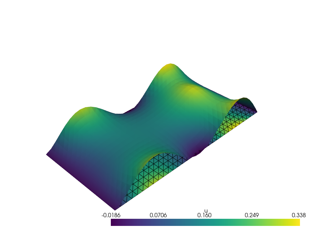
运行结果
dolfin代码实现
from dolfin import *
# Set pressure function:
T = 10.0 # tension
A = 1.0 # pressure amplitude
R = 0.3 # radius of domain
theta = 0.2
x0 = 0.6*R*cos(theta)
y0 = 0.6*R*sin(theta)
sigma = 0.025
#sigma = 50 # large value for verification
n = 40 # approx no of elements in radial direction
mesh = UnitCircle(n)
V = FunctionSpace(mesh, "Lagrange", 1)
# Define boundary condition w=0
def boundary(x, on_boundary):
return on_boundary
bc = DirichletBC(V, Constant(0.0), boundary)
# Define variational problem
w = TrialFunction(V)
v = TestFunction(V)
a = inner(nabla_grad(w), nabla_grad(v))*dx
f = Expression("4*exp(-0.5*(pow((R*x[0] - x0)/sigma, 2)) "\
" - 0.5*(pow((R*x[1] - y0)/sigma, 2)))",
R=R, x0=x0, y0=y0, sigma=sigma)
L = f*v*dx
# Compute solution
w = Function(V)
problem = LinearVariationalProblem(a, L, w, bc)
solver = LinearVariationalSolver(problem)
solver.parameters["linear_solver"] = "cg"
solver.parameters["preconditioner"] = "ilu"
solver.solve()
# Plot scaled solution, mesh and pressure
plot(mesh, title="Mesh over scaled domain")
plot(w, title="Scaled deflection")
f = interpolate(f, V)
plot(f, title="Scaled pressure")
# Find maximum real deflection
max_w = w.vector().array().max()
max_D = A*max_w/(8*pi*sigma*T)
print "Maximum real deflection is", max_D
# Verification for "flat" pressure (large sigma)
if sigma >= 50:
w_exact = Expression("1 - x[0]*x[0] - x[1]*x[1]")
w_e = interpolate(w_exact, V)
dev = numpy.abs(w_e.vector().array() - w.vector().array()).max()
print ’sigma=%g: max deviation=%e’ % dev
# Should be at the end
interactive()
新版本的dolfinx较老版本的dolfin更为麻烦,调的库更多(ps: 两份代码不是同一个方程, 只是用于演示二者接口的差异)。虽然dolfinx代码相对FreeFEM更麻烦,但好处是自由度更高,从函数空间定义到解\(Ax=b\)的线性方程组,都可以进行指定其细节。
这里对代码的运行时间进行简要分析:
| 步骤\单元格剖分 | (32, 16) | (64, 32) | (128, 64) | (256, 128) |
| 组装矩阵 | 0.003294 | 0.006112 | 0.023337 | 0.062674 |
| 解线性方程组 | 0.003260 | 0.006738 | 0.021041 | 0.120141 |
可以看出解线性方程组的速度是影响有限元计算的核心因素,其时间复杂度显著超过组装矩阵环节~
Comments | NOTHING